
The freezing point of a substance is the temperature at which its vapor pressure in its liquid phase equals its vapor pressure in its solid phase. When solutes are added, the freezing point of a solvent is lowered, which is referred to as the depression of the freezing point. It is a colligative property of solutions that is often proportional to the molality of the additional solute.
What is Freezing Point?
The temperature at which a substance transforms from a liquid state to a solid state is referred to as its freezing point. A substance’s melting point and freezing point are not always the same. Both the freezing and melting processes can be reversed.
Depression of Freezing Point
The phenomenon where a solution’s freezing point is lower than that of the pure solvent is known as “depression of freezing point,”.
Depression of freezing point is a collective property seen in solutions and is brought about by the addition of solute molecules to a solvent. The freezing points of solutions are all lower than that of the pure solvent and is directly proportional to the molality of the solute.
Why do the Depression of Freezing Point occurs?
The following explanation explains why the presence of a solute causes a solvent’s freezing point to decrease.
An equilibrium exists between the liquid and solid states of a solvent at its freezing point. According to this, the liquid and solid phases have the same vapor pressures.
The solution’s vapor pressure is discovered to be lower than the pure solvent’s vapor pressure after the addition of a non-volatile solute. As a result, the solid and solution attain equilibrium at lower temperatures.
Examples of Depression of Freezing Point
- The freezing temperature of ice is lowered and ice crystal formation is controlled when salt is added to the ice prior to making ice cream. Depression of freezing point is the reason behind this.
- Applying salt to snow-covered roads aids in lowering the freezing point of water, causing the ice to melt and clearing the road of snow.
- Most high-proof alcoholic drinks don’t freeze in a household freezer, including vodka. However, the freezing point (-173.5°F or -114.1°C) is higher than that of pure ethanol. It’s possible to think about vodka as an ethanol-in-water solution.
Depression of Freezing Point Equation
The curve ABC in the figure below shows how the vapor pressure of a pure liquid changes with temperature. At B, where the freezing-point curve actually starts, there is a sharp break. As a result, point B is equivalent to Tf, the freezing point of a pure solvent. The vapour pressure curve of a solution (solution 1) of a nonvolatile solute in the same solvent is also depicted in figure. It is comparable to the pure solvent’s vapour pressure curve and intersects the freezing point curve at F, showing that T1 is the freezing point of the solution.
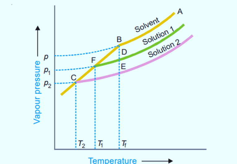
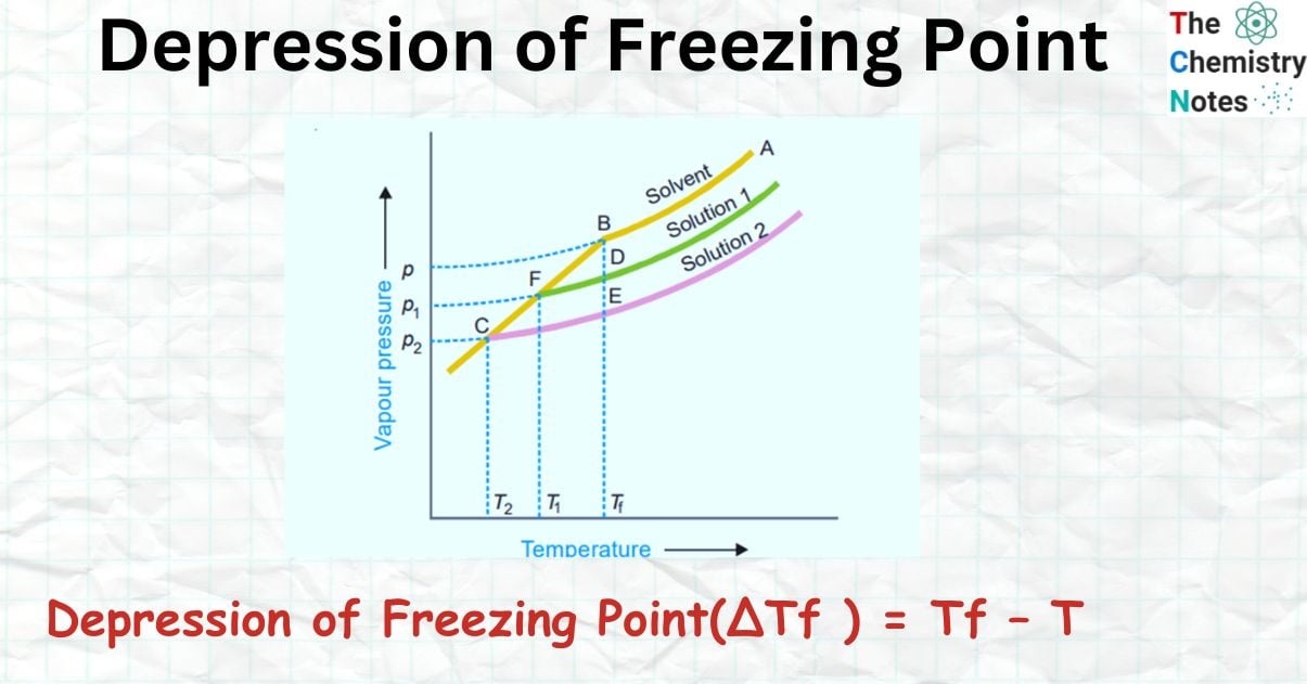
The difference in freezing points between the pure solvent and the solution is known as the Depression of freezing point. It is denoted by the sign ΔT or ΔTf.
ΔTf = Tf – T
When we add more solute to solution 1, we get a more concentrated solution (solution 2). The vapour pressure of solution 2 meets the freezing point at C, suggesting that the freezing point has been lowered to T2.
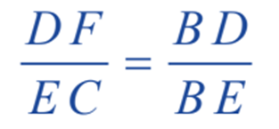
For dilute solutions, the straight lines FD and CE are nearly parallel, and BC is also a straight line. Given that BDF and BEC are similar triangles.
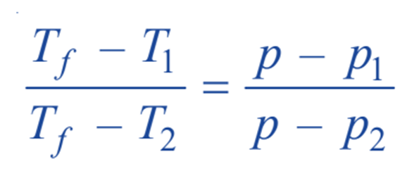
where p1 and p2 are vapour pressure of solution 1 and solution 2 respectively.
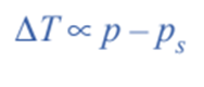
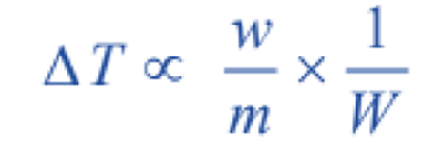
Hence, from above expression, depression of freezing point is directly proportional to the lowering of vapour pressure.
Determination of Molecular Weight from Depression of Freezing Point
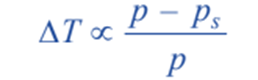
Since p is constant for the same solvent at a fixed temperature, we can write above equation as;
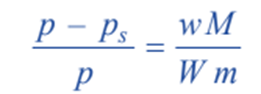
But from Raoult’s Law for dilute solutions,
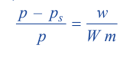
Since M (mol wt) of solvent is constant, above equation can be written as;
Solving the equations;
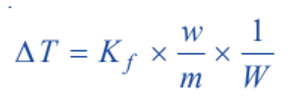
where,
Kf is a constant called Freezing-point constant or Cryoscopic constant or Molal depression constant.
If w/m = 1 and W = 1, Kf = ΔT. Thus,
Molal depression constant may be defined as the freezing-point depression produced when 1 mole of solute is dissolved in one kg (1000 g) of the solvent.
If the mass of solvent (W) is given in grams, it has to be converted into kilograms. Thus the expression assumes the form;
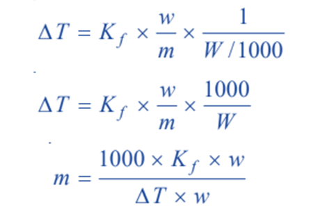
where;
m = molecular mass of solute ; Kf = molal depression constant ; w = mass of solute ;
ΔT = depression of freezing point ; W = mass of solvent.
Given the value of Kf , the molecular mass of solute can be calculated.
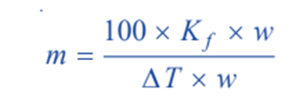
Sometimes the value of Kf is given in K per 0.1 kg. (100 g.) In that case, the expression
becomes;
The value of Kf: The value of Kf can be determined by measurement of ΔT by taking a solute of known molecular mass (m) and substituting the values in expression. The constant Kf, which is characteristic of a particular solvent, can also be calculated from the relation;
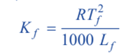
where Tf= freezing point of solvent in K; Lf= molar latent heat of fusion; R = gas constant.
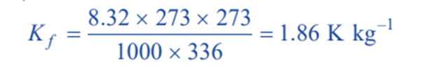
Hence for water, Tf = 273 K and Lf = 336 J g–1. Therefore;
Molal Depression constant for some common solvents
| Solvent | Kf per kg (1000 g) | Kf per 0.1 kg (100 g) |
| Water | 1.86 | 18.6 |
| Ethanoic acid (acetic acid) | 3.90 | 39.0 |
| Benzene | 5.10 | 51.0 |
| Camphor | 40.0 | 400.0 |
Measurement of Depression of Freezing Point
The freezing point depression can be determined more accurately and easily. The following are two easy ways that are often utilized.
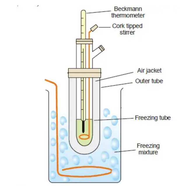
Beckmann’s Method
Apparatus: It consists of:
- A freezing tube with a side arm to hold the solvent or solution while the solute is delivered through the side arm;
- An outer bigger tube into which the freezing tube is fitted, with the gap in between providing an air jacket to ensure a slower and more uniform rate of cooling.
- A large jar containing a freezing mixture e.g., ice and salt, and having a stirrer.
Procedure:
- 15 to 20 g of the solvent is taken in the freezing point of the solvent by directly coding the freezing point tube Note: the bulb of the thermometer should be entirely immersed in the solvent.
- First, determine the approximate freezing point of the solvent by directly cooling the freezing point tube in the cooling bath.
- After that, melt the solvent and place the freezing-point tube back in the freezing bath, allowing the temperature to decline.
- When the temperature has dropped to within a degree of the approximate freezing point determined above, dry the tube and carefully place it in the air jacket.
- Allow the temperature to gradually drop, and then vigorously stir until it has dropped to roughly 0.5° below the freezing point.
- As a result of the latent heat being released, the solid will separate and the temperature will rise.
- Take note of the greatest temperature obtained and repeat the process to obtain a concordant freezing point value.
- After properly determining the solvent’s F.P, the solvent is remelted by removing the tube from the bath, and a weighed amount (0.1-0.2 g) of the solute is supplied through the side tube.
- The freezing point of the solution is now determined in the same way that the freezing point of the solvent is.
- After that, another amount of solute can be added and another reading taken.
- Knowing the freezing point depression, the molecular weight of the solute can be calculated using the expression of depression of freezing point.
References
- Atkins, Peter and de Paula, Julio. Physical Chemistry for the Life Sciences. New York, N.Y.: W. H. Freeman Company, 2006. (124-136).
- Laidler, K.J.; Meiser, J.L. (1982). Physical Chemistry. Benjamin/Cummings. ISBN 978-0618123414
- https://readchemistry.com/2022/09/14/measurement-of-freezing-point-depression/
- https://qsstudy.com/measurement-depression-freezing-point/
- T. Engel and P. Reid, Physical Chemistry (Pearson Benjamin Cummings 2006
- Tro, Nivaldo J. (2018). Chemistry: Structure and Properties (2nd ed.). Pearson Education. ISBN 978-0-134-52822-9.
- McQuarrie, Donald, et al. Colligative properties of Solutions” General Chemistry Mill Valley: Library of Congress, 2011. ISBN 978-1-89138-960-3.