
Errors and uncertainty are the two basic outcomes of any measurement carried out. Almost every scientific measurement and experiment involves measuring physical quantities such as length, mass, time, temperature, current, voltage, force, or volume. However, no physical measurement can give a perfect outcome. Every measurement has some degree of limitation. This may occur because measuring instruments are of finite precision, experimental conditions may change, and human observations are not completely perfect. For this reason, errors and uncertainties are included when reporting experimental results.
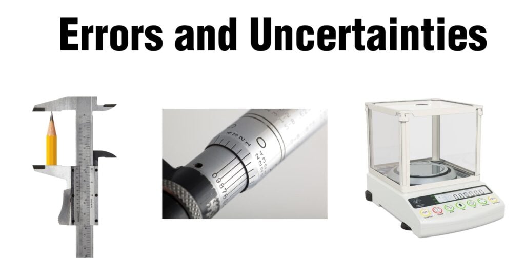
Errors and uncertainties do not always mean that the experiment performed was a failure. Instead, they are an essential part of scientific measurement. An experiment not having even a small amount of error is not considered a realistic one. Hence, the estimated value is always attached with an expected error.
For example, if the length of an object is measured as
L=(25.4±0.1) cm,
the value 25.4 cm is the measured value, while ±0.1 cm represents the uncertainty associated with the measurement.
Understanding errors and uncertainties is therefore important while interpreting our result and knowing the significance of the experiment conducted.
What Are Errors and Uncertainties?
After conducting the measurement and calculations, the measured value can deviate slightly or largely from the true or standard value. This difference between the two values is called an error. Mathematically, we write error as,
Error = xm−xt
Where xm is the measured value and xt is the true value.
There are also many experiments in practical life where the true value is unknown or may not be exact. Hence, the actual error is difficult to determine. Instead, scientists estimate the uncertainty associated with a measurement.
Uncertainty is the range within which the true value is expected to lie. It gives the degree of deviation of the outcome from the true value.
For example, if a mass is recorded to have the value,
m=(50.0±0.5) g
It means that the uncertainty of mass measurement is approximately 0.5 g. Also, we say that the actual value is close to the range 49.5 g to 50.5 g. It depends on how the uncertainty has been estimated. The uncertainty in measurement doesn’t mean that our measurement is wrong. It only emphasizes that measurement cannot give unlimited information.
Every measuring instrument has a resolution or smallest scale division. For example, a ruler marked in millimetres cannot give micrometer measurements precisely. Some various reasons for uncertainties in measurement are:
- limitations of measuring instruments,
- calibration problems,
- environmental changes,
- variations in experimental conditions,
- human observation,
- limitations of the experimental method,
- and random variations between repeated measurements.
The purpose of uncertainty analysis is to identify these limitations and communicate them clearly.
Types of Errors in Measurement
Measurement errors are of two types: systematic errors and random errors.
These errors behave differently and therefore require different approaches for their reduction.
A systematic error tends to affect measurements in a consistent manner. It may lead the measurement to be too large or too small, but the result is consistent.
On the other hand, a random error makes the measurement unpredictable, i.e, two simultaneous measurements of the same physical quantity can have a vast difference. Also, the same measurement can result in a slightly greater value at one time and slightly lower on another.
For example, if the length of a string is noted as:
3.2 cm, 3.3 cm, 3.1 cm, 3.2 cm.
The small differences between the readings can be called a random error.
However, if the ruler has already got defects in its manufacturing such that it shows 1 cm extra, the readings might be:
4.2 cm, 4.3 cm, 4.1 cm, 4.2 cm.
In this case too, the readings appear close to each other, and we call them precise, but they have a constant variation from the true value due to the device’s defect. This is an example of systematic error.
The difference between these two errors must be understood carefully because random error can be reduced but systematic error cannot be removed in general.
Systematic Errors
A systematic error is an error that produces a consistent bias in measurements. It often affects all measurements in a similar way.
Systematic errors can have several causes.
Instrumental Errors
Instrumental error occurs due to some defects on the measuring device itself or if it is not calibrated properly. For example, if a pan balance shows 0.2 g even when nothing is placed on it, we call it an error called a zero error. Every time we measure a mass, we get this error if the device is not fixed.
Environmental Errors
Sometimes our changing surroundings can also bring systematic errors, which are called environmental errors.
For example, changing temperature can slightly affect the length of metal rods. If an experiment is performed at a temperature different from the calibration temperature of the instrument, the result may be systematically affected.
Other environmental factors can include:
- temperature,
- atmospheric pressure,
- humidity,
- vibrations,
- magnetic fields,
- and electrical interference.
Experimental or Methodological Errors
The experimental procedure itself can sometimes create a systematic error.
For example, suppose the volume of liquid in a container is consistently read from the wrong position. Every measurement may then be biased in the same direction.
Similarly, if a measuring device is positioned incorrectly during an experiment, all the results may be affected.
Observational Errors
Human observation can also produce systematic errors. A common example is parallax error.
When reading a scale, the observer should position their eye directly in line with the measurement. If the scale is viewed from an angle, the apparent position of the pointer or liquid level may be incorrect.
Systematic errors are especially important because simply repeating the measurement does not normally solve the problem. If the same faulty instrument or procedure is used repeatedly, the same systematic error remains.
To reduce systematic errors, scientists may:
- calibrate instruments,
- correct zero errors,
- use standard reference values,
- improve experimental procedures,
- control environmental conditions,
- and compare results using an independent measurement method.
Random Errors
Random errors are unpredictable errors. So, no matter how many times we repeat our experiment, each time we get inconsistent results. They can occur due to the limitations in the measuring device, or personal negligence while recording data or performing the experiment.
For example, we are measuring the time taken by a ball to reach the ground using a stopwatch. Several trials might give:
1.21 s,1.25 s,1.19 s,1.23 s,1.22 s.
The differences between the readings may occur because the exact starting and stopping times are difficult to determine.
Unlike systematic errors, random errors do not consistently shift the results in one direction. Some measurements may be higher and others lower than the average.
One of the most effective ways of reducing random uncertainty is to repeat the measurement several times and calculate the average.
The mean is given by
xˉ=nx1+x2+x3+⋯+xn.
For example, suppose three measurements of a length are:
10.2 cm,10.4 cm,10.3 cm.
The mean is
xˉ=310.2+10.4+10.3 xˉ=10.3 cm.
The average gives a better estimate of the measured quantity than relying on a single reading, provided that the variations are genuinely random.
However, repeating measurements does not eliminate systematic errors. If an instrument consistently gives readings that are too high, taking hundreds of measurements with the same instrument will simply produce a very precise but inaccurate result.
Accuracy and Precision
Accuracy and precision are two common terms in measurement that are related to each other but different in concept.
Accuracy shows a relation between the true value and the measured value, while precision shows the relation between the values of the same repeated measurements. Suppose the accepted value of a quantity is 50.0. To make it clear, let us describe three cases:
Case 1: Accurate and precise
Readings:
49.9,50.0,50.1,50.0
Here, the measured value is close to the accepted value, and also, on repeating the experiment, we get close readings. Hence, our measurement is both accurate and precise.
Case 2: Precise but inaccurate
Readings:
47.2,47.2,47.3,47.2
The readings are very close to one another but differ a lot from the accepted value. So the measurement is precise but not accurate. This can happen if the measuring device has some defects and causes systematic error.
Case 3: Accurate on average but not precise
Readings:
46,54,49,51
The readings differ very much from the accepted value and are also inconsistent on repeated measurements. This can give a close value on average but is not precise.
A good scientific experiment aims to achieve both high accuracy and high precision.
Precision is strongly related to the resolution of the instrument and the size of random variations, while accuracy is strongly affected by systematic errors.
Absolute, Fractional, and Percentage Uncertainty
Uncertainties are basically of three types: absolute uncertainty, fractional uncertainty, and percentage uncertainty.
Absolute Uncertainty
Absolute uncertainty is expressed in the same units as the measured quantity.
For example:
L=(40.0±0.5) cm.
The absolute uncertainty is:
0.5 cm
The result tells us that the measurement has an approximate uncertainty of 0.5 cm.
Absolute uncertainty directly shows the range of uncertainty.
Fractional Uncertainty
Fractional uncertainty compares the absolute uncertainty with the measured value.
It is calculated using:
Fractional uncertainty=Measured valueAbsolute uncertainty.
For a measurement of
L=40.0±0.5 cm,
the fractional uncertainty is
0.5/40.0 = 0.0125.
Therefore, the fractional uncertainty is:
0.0125.
Fractional uncertainty has no units.
Percentage Uncertainty
Percentage uncertainty is the expression of fractional uncertainty as a percentage.
Percentage uncertainty = Absolute uncertainty / Measured Value ×100%.
From the above example of fractional uncertainty, we can write,
Percentage uncertainty = 0.5/40.0×100% =1.25%.
So, we can write that the measurement has a percentage uncertainty of approximately 1.25%.
Percentage uncertainty is particularly useful when comparing measurements.
Uncertainty in Derived Quantities
In science, many quantities are not measured directly. Instead, they are calculated using other measured quantities.
For example, the area of a rectangle is calculated as:
A = length × width.
On measuring, length and width may contain some uncertainties. Therefore, the calculated area will also bear some uncertainty.
There are various methods to find this combined uncertainty.
Addition and Subtraction
When quantities are added or subtracted, their absolute uncertainties are generally added.
If
Q=A+B,
then
ΔQ=ΔA+ΔB.
For example, suppose
A=20.0±0.2
and
B=10.0±0.1.
Then:
Q=30.0
and the uncertainty is:
ΔQ=0.2+0.1=0.3.
Therefore:
Q=30.0±0.3.
Multiplication and Division
For multiplication and division, fractional or percentage uncertainties are generally added.
If
Q=AB,
then approximately:
ΔQ/Q = ΔA/A + ΔB/B.
The same general rule applies to division.
For example, suppose a rectangle has:
l=20.0±0.2 cm
and
w=10.0±0.1 cm.
The area is:
A=20.0×10.0=200 cm2.
The fractional uncertainty is approximately:
0.2/20.0 +0.1/10.0 = 0.01+0.01 =0.02.
Therefore, the percentage uncertainty is:
0.02×100%=2%.
The approximate absolute uncertainty in area is:
0.02×200=4 cm2.
Thus, the area can be reported approximately as:
A=(200±4) cm2.
Quantities Raised to a Power
If a quantity is raised to a power, the fractional uncertainty is multiplied by that power.
For:
Q=An,
the approximate fractional uncertainty is:
ΔQ/Q = |n|ΔA/A.
For example, the volume of a sphere is:
V = 4/3πr3.
As the radius is the cube of r, the uncertainty in radius is multiplied by 3.
Therefore, it is important to be careful while calculating fractional uncertainties for the quantities raised to powers.
Reducing Errors and Improving Accuracy
Errors cannot be eliminated from the measurements but can be reduced if performed carefully. The following tips can be followed:
Use Appropriate Measuring Instruments
The range and resolution of the measuring device should be selected correctly. For example, a meter scale cannot measure a small spherical metallic ball. Hence, a micrometer screw gauge can give accurate measurements.
Calibrate Instruments
Instruments should be checked against a standard device before using them. Calibration can prevent systematic errors, and the measurement can be reliable.
Check for Zero Errors
The zero position of the device must be checked before operating it. If the instrument already has a zero error, the device must be corrected accordingly.
Repeat Measurements
Repeating measurements helps reduce the influence of random errors. Several readings can be taken and averaged.
However, repeated measurements are most useful when they are independent, and the experimental conditions remain appropriate.
Avoid Parallax
When reading an analogue scale, the observer’s eye should be positioned directly in line with the pointer or liquid level. This reduces parallax error.
For liquid measurements, the correct part of the meniscus should also be read according to the experimental procedure.
Control Environmental Conditions
If environmental conditions like temperature, pressure, humidity, vibration, etc., are likely to affect the experiment, the factors must be eliminated or noted.
For example, a fan can affect the experiment performed to verify the law of moments that needs a balanced condition.
Improve Experimental Design
A carefully designed experiment can significantly reduce uncertainty.
This may involve:
- using larger measurable quantities,
- increasing the number of observations,
- selecting better instruments,
- reducing unnecessary variables,
- controlling experimental conditions,
- and choosing a measurement method that minimizes uncertainty.
For example, if measuring the time for a single oscillation of a pendulum produces a large timing uncertainty, measuring the time for many oscillations and then dividing by the number of oscillations can reduce the relative effect of reaction-time uncertainty.
Report Results Honestly
Scientific results should not appear more precise than the measurements justify.
If an instrument provides measurements reliable only to the nearest 0.1 unit, reporting a result such as 15.372846 units would suggest a level of precision that was not actually obtained.
Results should therefore be reported using appropriate significant figures and with a realistic uncertainty.
Conclusion
Measurement cannot fully eliminate errors and uncertainties. Therefore, they are also an important part of measurement which cannot be discarded. Thus, they must be recognized, and it will be best to inform about the errors and expected uncertainties. Steps are always taken to make the error as low as possible.
Two different errors- systematic and random errors can occur in our measurement. Systematic error is due to errors already in the device or weaknesses in experimental methods, while random error occurs due to human errors or limitations of the device. Systematic error cannot be removed, while random errors can be removed by handling the experiment carefully, repeatedly, or taking an average.
Accuracy and precision are two major concepts for conducting a good measurement. Accurate measurement seeks closeness to the true value, while a precise measurement seeks closeness in the repeated measurement values. Both are equally important to reduce errors and uncertainties to a maximum.
Uncertainties are also three types: absolute uncertainty, fractional uncertainty, or percentage uncertainty. These forms allow scientists to describe the reliability of measurements and compare the quality of different experimental results. When measured quantities are used to calculate derived quantities, their uncertainties must also be considered and combined appropriately.
A good scientific measurement clearly talks about these errors, uncertainties, and limitations of the devices. They are also reported honestly and are tried to keep them low. A result accompanied by a well-understood uncertainty is far more scientifically useful than a seemingly exact number with no indication of its reliability.
References
- Taylor, J. R. (2022). An introduction to error analysis: the study of uncertainties in physical measurements. MIT Press.
- Hughes, I., & Hase, T. (2010). Measurements and their uncertainties: a practical guide to modern error analysis. Oup Oxford.
- Fornasini, P. (2008). The uncertainty in physical measurements: an introduction to data analysis in the physics laboratory. New York, NY: Springer New York.
- Cohen, E. R. (1998). An introduction to error analysis: The study of uncertainties in physical measurements. Measurement Science and Technology, 9(6), 022.
- https://www.physics.columbia.edu/sites/www.physics.columbia.edu/files/content/Lab%20Resources/Lab%20Guide%201_%20Introduction%20to%20Error%20and%20Uncertainty.pdf
- https://phys.libretexts.org/Courses/Georgia_State_University/GSU-TM-Physics_I_(2211)/01%3A_Introduction_to_Physics_Measurements_and_Mathematics_Tools/1.03%3A_Measurements_Uncertainty_and_Significant_Figures
- https://physmatica.com/physics/measurement-uncertainty
